Lid-driven cavity

Standard CFD benchmark, which allows comparison with very accurate mesh-based methods. Description of the problem can be found on many webpages, like here. In the image below, you can see streamlines for Re = 400 and N = 320. This was computed on cluster and took some time. To correctly resolve corner vortices is much more demanding in SPH than in FEM.

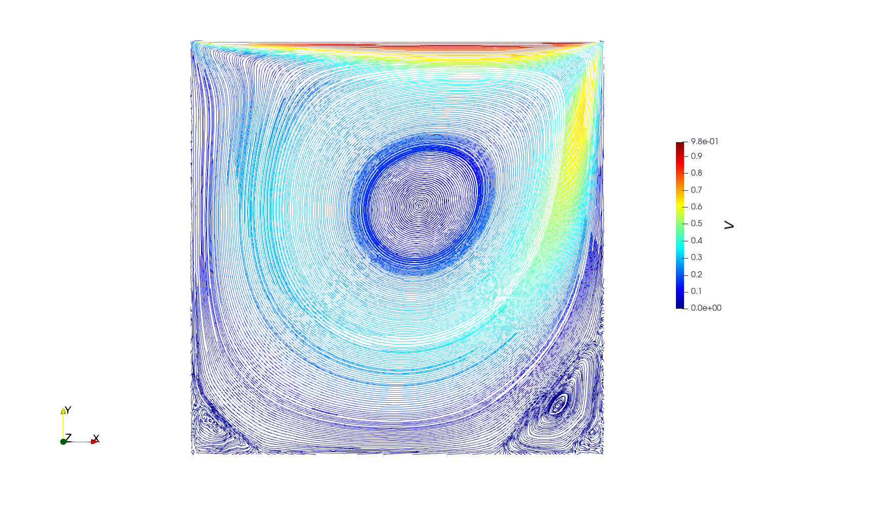
Result is compared to the referential solution by Ghia et al 1980.

module cavity_flow

using Printf
using SmoothedParticles
using Plots, CSV, DataFrames, Printf, LaTeXStrings, Parameters

Declare const parameters (dimensionless problem)

##geometrical/physical parameters
const N  =   100                #number of sample points
const Re =   100                #Reynolds number
const llid = 1.0                #length of the lid
const mu =   1.0/Re             #viscosity
const rho0 = 1.0                #density
const vlid = 1.0                #flow speed of the lid
const dr = llid/N 		        #interparticle distance
const h = 3.0*dr		        #size of kernel support
const m = rho0*dr^2             #particle mass
const c = 20*vlid		    	#numerical speed of sound
const P0 = 5.0                  #background pressure (good to prevent tensile instability)
const wwall = h

##temporal parameters
const dt = 0.1*h/c                       #numerical time-step
const t_end = 0.4                        #end of simulation
const dt_frame = max(dt, t_end/200)      #how often save data

##particle types
const FLUID = 0.
const WALL = 1.
const LID = 2.

##path to store results
const path = "results/cavity_flow"*string(Re)

Declare variables to be stored in a Particle

@with_kw mutable struct Particle <: AbstractParticle
	x::RealVector=VEC0	#position
	v::RealVector=VEC0  #velocity
	Dv::RealVector=VEC0 #acceleratation
	rho::Float64=rho0   #density
	Drho::Float64=0.0   #rate of density
	P::Float64=0.0      #pressure
	type::Float64       #particle type
end

Define geometry and create particles

function make_system()
	grid = Grid(dr, :hexagonal)
	box = Rectangle(0., 0., llid, llid)
	wall = BoundaryLayer(box, grid, wwall)
	sys = ParticleSystem(Particle, box + wall, h)
	lid   = Specification(wall, x -> x[2] > llid)
	wall = Specification(wall, x -> x[2] <= llid)
	generate_particles!(sys, grid, box, x -> Particle(x=x, type=FLUID))
	generate_particles!(sys, grid, lid, x -> Particle(x=x, type=LID))
	generate_particles!(sys, grid, wall, x -> Particle(x=x, type=WALL))
	create_cell_list!(sys)
	apply!(sys, find_pressure!)
	apply!(sys, internal_force!)
	return sys
end

Define interactions between particles

function balance_of_mass!(p::Particle, q::Particle, r::Float64)
	p.Drho += m*rDwendland2(h,r)*(dot(p.x-q.x, p.v-q.v))
end

function find_pressure!(p::Particle)
	p.rho += p.Drho*dt
	p.Drho = 0.0
	p.P = P0 + c^2*(p.rho-rho0)
end

function internal_force!(p::Particle, q::Particle, r::Float64)
	rDk = rDwendland2(h,r)
	x_pq = p.x - q.x
	v_pq = p.v - q.v

implementation of the Dirichlet boundary condition at the lid v_q is estimated using linear extrapolation

	if q.type == LID
        s = abs(x_pq[2])/(0.1*h + abs(p.x[2] - 1.0))
        v_pq = s*(p.v - vlid*VECX)
    end
	p.Dv += -m*rDk*(p.P/p.rho^2 + q.P/q.rho^2)*x_pq
	p.Dv += 8/(Re*p.rho*q.rho)*m*rDk*dot(v_pq, x_pq)/(r^2 + 0.01*h^2)*x_pq #Monaghan's type of viscosity to conserve angular momentum
end


function move!(p::Particle)
	p.Dv = VEC0
	if p.type == FLUID
		p.x += 0.5*dt*p.v
	end
end

function accelerate!(p::Particle)
	if p.type == FLUID
		p.v += 0.5*dt*p.Dv
	end
end

Time iteration

function main()
	sys = make_system()
	out = new_pvd_file(path)
	@time for k = 0 : Int64(round(t_end/dt))
		apply!(sys, accelerate!)
		apply!(sys, move!)
		create_cell_list!(sys)
		apply!(sys, balance_of_mass!)
		apply!(sys, find_pressure!)
		apply!(sys, move!)
		create_cell_list!(sys)
		apply!(sys, internal_force!)
		if (k % Int64(round(dt_frame/dt)) == 0) #save the frame
			@printf("t = %.6e s ", k*dt)
			println("(",round(100*k*dt/t_end),"% complete)")
			save_frame!(out, sys, :P, :v, :type)
		end
		apply!(sys, accelerate!)
	end
	save_pvd_file(out)
	compute_fluxes(sys)
	make_plot()
end

Functions to extract results and create plots.

function compute_fluxes(sys::ParticleSystem, res = 100)
    s = range(0.,1.,length=res)
    v1 = zeros(res)
    v2 = zeros(res)
    for i in 1:res
		#x-velocity along y-centerline
		x = RealVector(0.5, s[i], 0.)
		gamma = SmoothedParticles.sum(sys, (p,r) -> Float64(p.type==FLUID)*m*wendland2(h,r), x)
        v1[i] = SmoothedParticles.sum(sys, (p,r) -> Float64(p.type==FLUID)*m*p.v[1]*wendland2(h,r), x)/gamma
		#y-velocity along x-centerline
		x = RealVector(s[i], 0.5, 0.)
		gamma = SmoothedParticles.sum(sys, (p,r) -> Float64(p.type==FLUID)*m*wendland2(h,r), x)
        v2[i] = SmoothedParticles.sum(sys, (p,r) -> Float64(p.type==FLUID)*m*p.v[2]*wendland2(h,r), x)/gamma
    end
    #save results into csv
    data = DataFrame(s=s, v1=v1, v2=v2)
	CSV.write(path*"/data.csv", data)
	make_plot()
end

function make_plot(Re=Re)
	ref_x2vy = CSV.read("reference/ldc-x2vy.csv", DataFrame)
	ref_y2vx = CSV.read("reference/ldc-y2vx.csv", DataFrame)
	propertyname = Symbol("Re", Re)
	ref_vy = getproperty(ref_x2vy, propertyname)
	ref_vx = getproperty(ref_y2vx, propertyname)
	ref_x = ref_x2vy.x
	ref_y = ref_y2vx.y
	data = CSV.read(path*"/data.csv", DataFrame)
	p1 = plot(
		data.s, data.v2,
		xlabel = L"x",
		ylabel = L"v_y",
		label = "SPH",
		linewidth = 4,
		legend = :bottomleft,
		color = :orange,
		tickfontsize = 16,
		labelfontsize = 16,
		legendfontsize = 16,
		aspect_ratio = 1,
	)
	scatter!(p1, ref_x, ref_vy, label = "REF", markershape = :diamond, ms = 5, color = :blue)
	savefig(p1, path*"/ldc-x2vy.pdf")
	p2 = plot(
		data.v1, data.s,
		xlabel = L"v_x",
		ylabel = L"y",
		label = "SPH",
		linewidth = 4,
		legend = :bottomright,
		color = :orange,
		tickfontsize = 16,
		labelfontsize = 16,
		legendfontsize = 16,
		aspect_ratio = 1,
	)
	scatter!(p2, ref_vx, ref_y,  label = "REF", markershape = :diamond, ms = 5, color = :blue)
	savefig(p2, path*"/ldc-y2vx.pdf")
end

end

This page was generated using Literate.jl.