Example 2: Lid-driven cavity

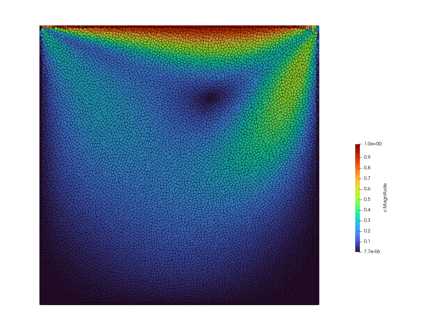
Simulation of a vortex induced by viscosity. The domain is a square

$\Omega = [0,1] \times [0,1]$

with Dirichlet boundary conditions everywhere. The sides and bottom are no-slip condition

$\mathbf{v} = 0, \quad \mathbf{x} \in \Gamma_\mathrm{left}\cup \Gamma_\mathrm{right} \cup \Gamma_\mathrm{bottom}.$

whereas the top side prescribes a uniform velocity in horizontal direction:

$\mathbf{v} = \begin{pmatrix} 1 \\ 0 \end{pmatrix}, \quad \mathbf{x} \in \Gamma_\mathrm{up}.$

The fluid is described by incompressible Navier-Stokes. The solution should be a steady flow, be we can reach it with a dynamic solver by setting sufficiently large t_end. To plot streamlines, open the pvd file in paraview and use the Evenly Spaced Streamlines filter.

module cavity
include("../src/LagrangianVoronoi.jl")
using .LagrangianVoronoi, DataFrames, CSV, Plots

We will use a strictly incompressible model but using the stiffened gas model with large initial sound speed like c0 = 1e3 is also fine.

const Re = 100 # Reynolds number
const N = 100 # resolution
const dr = 1.0/N
const dt = min(0.1*dr, 0.1*Re*dr^2)
const t_end = 0.1*Re
const export_path = "results/cavity/Re$Re"
const rho0 = 1.0 # fluid density

Define the boundary condition for velocity and the initial condition. We must specify the density, mass and the dynamic coefficient of viscosity. To get incompressible fluid, we set the initial sound speed (squared) to plus infinity.

function vDirichlet(x::RealVector)::RealVector
    islid = isapprox(x[2], 1.0, atol = 0.1dr)
    return islid ? VECX : VEC0
end

function ic!(p::VoronoiPolygon)
    p.rho = rho0
    p.mass = p.rho*area(p)
    p.mu = 1.0/Re
    p.c2 = Inf
end

mutable struct Simulation <: SimulationWorkspace
    grid::GridNS
    mesh_quality::Float64
    energy::Float64
    solver::PressureSolver{PolygonNS}
    Simulation() = begin
        domain = UnitRectangle()
        grid = GridNS(domain, dr)
        populate_lloyd!(grid, ic! = ic!)
        return new(grid, 0.0, 0.0, PressureSolver(grid))
    end
end

When defining the step, we need to activate boundary friction. We omit the equation of state as there is no such thing in the incompressible regime.

function step!(sim::Simulation, t::Float64)
    move!(sim.grid, dt)
    find_pressure!(sim.solver, dt)
    pressure_step!(sim.grid, dt)
    find_D!(sim.grid)
    viscous_step!(sim.grid, dt; artificial_viscosity = false)
    bdary_friction!(sim.grid, vDirichlet, dt)
    find_dv!(sim.grid, dt)
    relaxation_step!(sim.grid, dt)
    return
end

function postproc!(sim::Simulation, t::Float64)
    sim.mesh_quality = Inf
    for p in sim.grid.polygons
        sim.energy += 0.5*p.mass*norm_squared(p.v)
        sim.mesh_quality = min(sim.mesh_quality, p.quality)
    end
    percent = round(100*t/t_end, digits = 5)
    println("sim time = $t ($(percent)%)")
    println("mesh quality = $(sim.mesh_quality)")
    println("kinetic energy = $(sim.energy)")
    println()
    return
end

Finally, we declare some functions to extract more data. Namely, we measure the horizontal velocity along the vertical axis and vice versa.

function compute_fluxes(grid::VoronoiGrid, res = 100)
    s = range(0.,1.,length=res)
    v1 = zeros(res)
    v2 = zeros(res)
    for i in 1:res
        #x-velocity along y-centerline
        x = RealVector(0.5, s[i])
        v1[i] = point_value(grid, x, p -> p.v[1])
        #y-velocity along x-centerline
        x = RealVector(s[i], 0.5)
        v2[i] = point_value(grid, x, p -> p.v[2])
    end
    #save results into csv
    data = DataFrame(s=s, v1=v1, v2=v2)
    CSV.write(joinpath(export_path, "vprofile_legacy.csv"), data)
    make_plot()
end

The plot of velocity is compared to a reference solution by Abdelmigid et al.

function make_plot()
    ref_x2vy = CSV.read("reference/ldc_x2vy_abdelmigid.csv", DataFrame)
    ref_y2vx = CSV.read("reference/ldc_y2vx_abdelmigid.csv", DataFrame)
    propertyname = Symbol("Re", Re)
    ref_vy = getproperty(ref_x2vy, propertyname)
    ref_vx = getproperty(ref_y2vx, propertyname)
    data = CSV.read(joinpath(export_path, "vprofile.csv"), DataFrame)
    plt = plot(
        data.s, [movingavg(data.v2) movingavg(data.v1)],
        xlabel = "x, y",
        ylabel = "u, v",
        label = ["v" "u"],
        linewidth = 2,
        legend = :topleft,
        color = [:orange :royalblue]
    )
    scatter!(plt,
        [ref_x2vy.x ref_y2vx.y], [ref_vy ref_vx],
        label = false,
        color = [:orange :royalblue],
        markersize = 4,
        markerstroke = stroke(1, :black),
        markershape = [:circ :square]
    )
    savefig(plt, joinpath(export_path, "vprofile.pdf"))
end

Finally, wrap everything into the function main.

function main()
    sim = Simulation()
    @time run!(
        sim,
        dt,
        t_end,
        step!;
        postproc! = postproc!,
        path = export_path,
        nframes = 200, # number of time frames
        vtp_vars = (:v, :P, :quality), # local variables exported in vtk
        csv_vars = (:energy, :mesh_quality) # global variables exported in csv
    )
    compute_fluxes(sim.grid)
    return
end

if abspath(PROGRAM_FILE) == @__FILE__
    main()
end

end

This page was generated using Literate.jl.