Example 7: Rayleigh-Bénard Instability
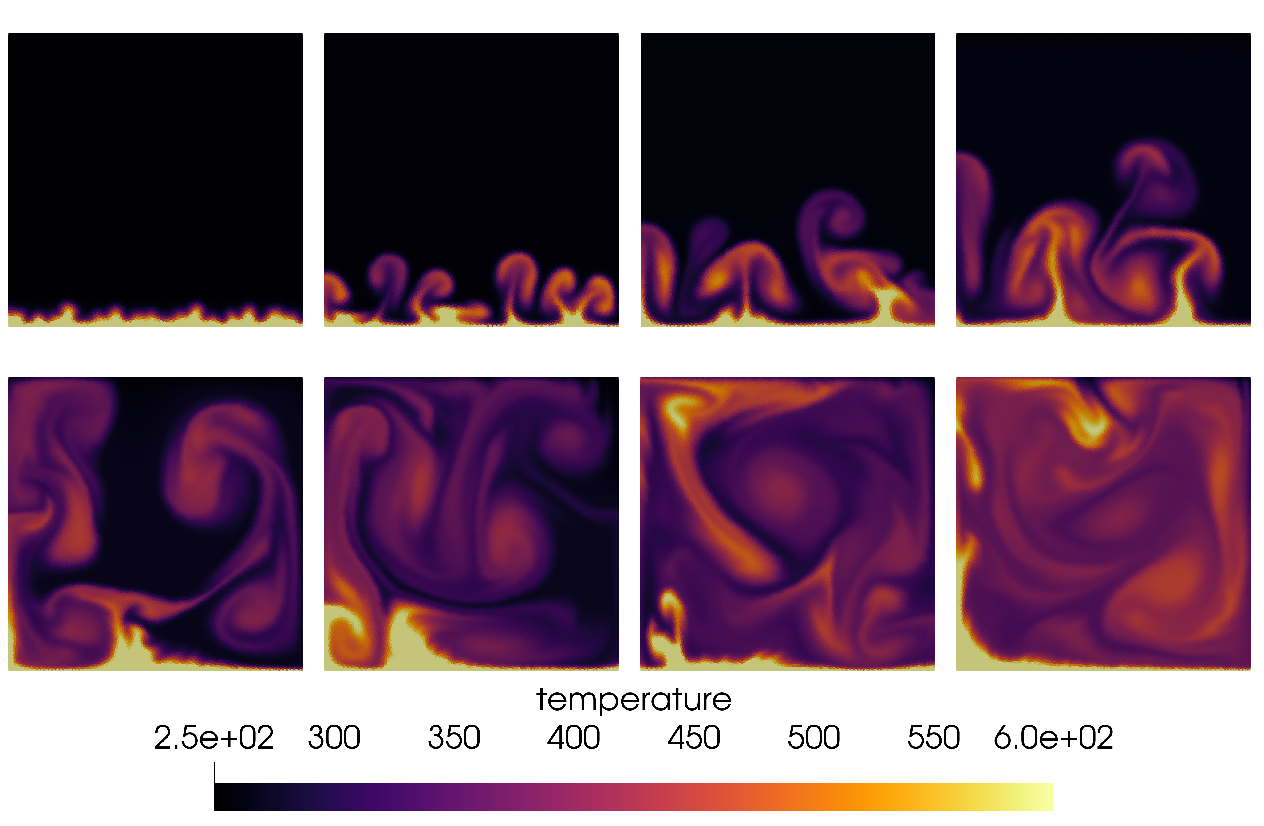
This test is similar to Rayleigh-Taylor but even more amazing. The top side of the domain is hot and the bottom is cold. The hot fluid expands and rises up, then cools again and sinks. The resulting dynamical pattern is called a convective cell. It is somehow related to atmosphere and weather. You can read more on wikipedia.
module heat
include("../src/LagrangianVoronoi.jl")
using .LagrangianVoronoi


const g = 9.8 #gravitation acceleration
const mu = 1e-4 #dynamic viscosity
const H = 0.1 #height
const W = 0.1
const gamma = 1.4 #adiabatic index
const rho0 = 10.0

const cV = 10.0  #sp. heat capacity
const R = (gamma - 1.0)*cV
const thermal_k = mu*cV*gamma/0.71 #thermal conductivity

const P0 = 1e4
const c0 = sqrt(gamma*P0/rho0)
const Tu = P0/(rho0*R) #temperature of upper boundary (cooler)
const Td = 1000.0 #30.0 #Tu*(1.0 + contrast) #temperature of lower boundary (heater)

const export_path = "results/heat"
const dr = H/100
const v_char = 2.0
const dt = 0.1*dr/v_char
const nframes = 400
const t_end = 1.0

function print_info()
    thermal_D = thermal_k/(rho0*gamma*cV) #thermal diffusivity
    thermal_a = 1.0/Tu
    nu = mu/rho0
    @show Pr = nu/thermal_D # Prandtl number
    @show Ra = thermal_a*g*(Td-Tu)*(H^3)/(nu*thermal_D) # Rayleigh number
end
Define the initial state (exponential atmosphere) and the boundary condition for temperature.
function exp_atmo!(p::VoronoiPolygon)
    p.T = Tu
    p.P = P0*exp(-g*p.x[2]/(R*Tu))
    p.e = cV*p.T
    p.rho = p.P/(R*p.T)
    p.mass = p.rho*area(p)
    p.k = thermal_k
    p.cV = cV
end

function T_bc(::RealVector, bdary::Int)::Float64
    if (bdary == BDARY_DOWN)
        return Td
    elseif (bdary == BDARY_UP)
        return Tu
    end
    return NaN # NaN indicates an adiabatic wall
end
The rest is fairly standard, except we also need to include Fourier diffusion in our time-marching scheme.
mutable struct Simulation <: SimulationWorkspace
    grid::GridNSF
    solver::PressureSolver{PolygonNSF}
    E::Float64
    S::Float64
    E_kinetic::Float64
    Simulation() = begin
        xlims = (0.0, W)
        ylims = (0.0, H)
        domain = Rectangle(xlims = xlims, ylims = ylims)
        grid = GridNSF(domain, dr, xperiodic = true)
        populate_lloyd!(grid, ic! = exp_atmo!)
        return new(grid, PressureSolver(grid), 0.0, 0.0, 0.0)
    end
end

function step!(sim::Simulation, t::Float64)
    move!(sim.grid, dt)
    gravity_step!(sim.grid, -g*VECY, dt)
    ideal_eos!(sim.grid, gamma)
    find_pressure!(sim.solver, dt)
    pressure_step!(sim.grid, dt)
    ideal_temperature!(sim.grid) # find the temperature according to ideal gas laws
    fourier_step!(sim.grid, dt)  # update the temperature by Fourier diffusion
    heat_from_bdary!(sim.grid, dt, T_bc, gamma) # add heat flux from boundaries
    find_D!(sim.grid)
    viscous_step!(sim.grid, dt)
    find_dv!(sim.grid, dt)
    relaxation_step!(sim.grid, dt)
    return
end

function postproc!(sim::Simulation, t::Float64)
    sim.S = 0.0
    sim.E = 0.0
    sim.E_kinetic = 0.0
    P0 = rho0*c0^2/gamma
    for p in sim.grid.polygons
        sim.S += p.mass*p.cV*(log(abs(p.P/P0)) - gamma*log(abs(p.rho/rho0)))
        sim.E += p.mass*p.e
        sim.E_kinetic += 0.5*p.mass*norm_squared(p.v)
    end
    percent = round(100*t/t_end, digits = 5)
    println("t = $t ($(percent)%)")
    @show sim.E
    @show sim.S
    @show sim.E_kinetic
    println()
end

function main()
    print_info()
    sim = Simulation()
    run!(sim, dt, t_end, step!; path = export_path,
        vtp_vars = (:v, :P, :T, :rho),
        postproc! = postproc!,
        nframes = nframes
    )
end

if abspath(PROGRAM_FILE) == @__FILE__
    main()
end

end
This page was generated using Literate.jl.