Example 1: Gresho Vortex Benchmark

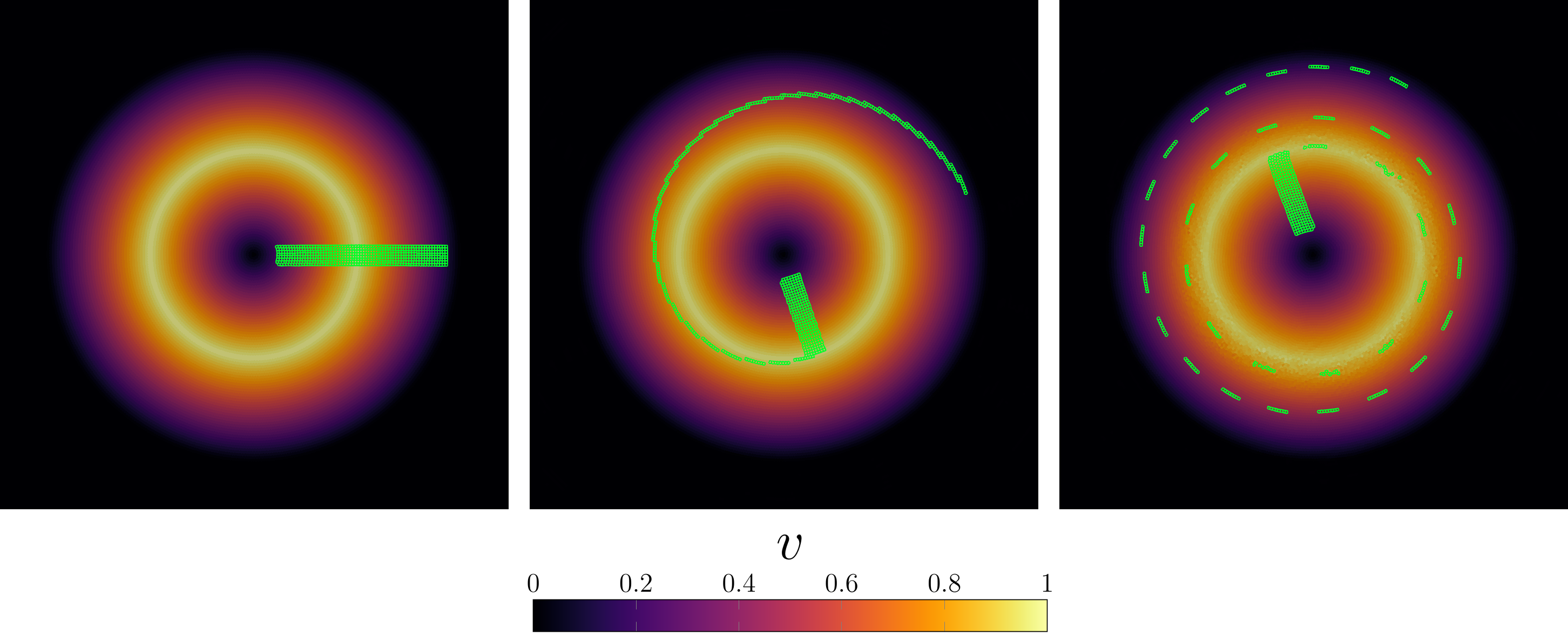
Gresho vortex is a very simple test which allows to compare a numerical solution to analytical result for arbitrary Mach number. The setup is a domain (usually square) with a prescribed vortex as the initial condition. The vortex should be steady in theory but it is not trivial to reproduce such behavior in a numerical code, especially since the initial condition is not a differentiable function.

Let us start by including LagrangianVoronoi module and importing some useful libraries.

module gresho
include("../src/LagrangianVoronoi.jl")
using .LagrangianVoronoi, WriteVTK, LinearAlgebra, Match
using LaTeXStrings, DataFrames, CSV, Plots, Measures

Declare constant parameters of the simulation. Especially the Mach number and the resolution.

const rho0 = 1.0 # initial density
const xlims = (-0.5, 0.5)
const ylims = (-0.5, 0.5)
const N = 100 # resolution
const dr = 1.0/N

const dt = 0.1*dr
const t_end =  1.0
const nframes = 100 # number of time frames (how many times we save the simulation state)

const Ma = 0.1 # Mach number
const c0 = 1.0/Ma # speed of sound
const gamma = 1.4 # adiabatic index
const stiffened = (c0 > 100) # do we use ideal or stiffened gas model?
const P0 = rho0*c0^2/gamma # initial density in the vortex core

const export_path = "results/gresho/Ma$Ma"

Define the exact solution, which is the same as initial condition.

function v_exact(x::RealVector)::RealVector
    omega = @match norm(x) begin
        r, if r < 0.2 end => 5.0
        r, if r < 0.4 end => 2.0/r - 5.0
        _ => 0.0
    end
    return omega*RealVector(-x[2], x[1])
end

function P_exact(x::RealVector)::Float64
    Pmin = (stiffened ? 0.0 : P0)
    return @match norm(x) begin
        r, if r < 0.2 end => Pmin + 12.5*r^2
        r, if r < 0.4 end => Pmin + 4.0 + 4*log(5*r) - 20.0*r + 12.5*r^2
        _ => Pmin - 2.0 + 4*log(2)
    end
end

This function enforces the inital condition on a VoronoiPolygon.

function ic!(p::VoronoiPolygon)
    p.v = v_exact(p.x) # velocity
    p.rho = rho0 # density
    p.mass = p.rho*area(p) # mass
    p.P = P_exact(p.x) # pressure
    p.e = 0.5*norm_squared(p.v) + p.P/(p.rho*(gamma - 1.0)) # internal energy
end

The Simulation worspace struct contains all simulation data, namely:

grid (and all local variables within)
pressure solver (allows us to solve an implicit system)
global (non-constant) variables

Polygons are generated in its constructor.

mutable struct Simulation <: SimulationWorkspace
    grid::GridNS
    solver::PressureSolver{PolygonNS}
    E::Float64  # total energy
    l2_err::Float64 # L^2 error
    Simulation() = begin
        domain = Rectangle(xlims = xlims, ylims = ylims)
        grid = GridNS(domain, dr)
        populate_circ!(grid, ic! = ic!)
        return new(grid, PressureSolver(grid), 0.0, 0.0)
    end
end

Function step! defines how simulation workspace changes when we update the time by dt. Number t is the simulation time before the update. We do not really need t but the module requires this argument.

function step!(sim::Simulation, t::Float64)
    move!(sim.grid, dt)
    if stiffened
        stiffened_eos!(sim.grid, gamma, P0) # stiffened gas equation of state
    else
        ideal_eos!(sim.grid, gamma) # ideal gas equation of state
    end
    find_pressure!(sim.solver, dt)
    pressure_step!(sim.grid, dt)
    find_D!(sim.grid)
    viscous_step!(sim.grid, dt)
    find_dv!(sim.grid, dt)
    relaxation_step!(sim.grid, dt)
    return
end

Function postproc!is called each time before the data is saved (much less often than step!). It can be used for post-processing but let's just print some information to the console.

function postproc!(sim::Simulation, t::Float64)
    sim.l2_err = 0.0
    sim.E = 0.0
    for p in sim.grid.polygons
        sim.l2_err += p.mass*norm_squared(p.v - v_exact(p.x))
        sim.E += p.mass*p.e
    end
    sim.l2_err = sqrt(sim.l2_err)
    percent = round(100*t/t_end, digits = 5)
    println("t = $t ($(percent)%)")
    println("energy = $(sim.E)")
    println("error = $(sim.l2_err)")
    println()
end

Wrap everything into the main function. Once the simulation ends, extract the velocity along midline and plot it.

function main()
    sim = Simulation()
    run!(sim, dt, t_end, step!;
        path = export_path,
        postproc! = postproc!,
        vtp_vars = (:v, :P),      # local variables exported into vtp
        csv_vars = (:E, :l2_err), # global variables exported into csv
        nframes = nframes         # number of time frames
    )
    vy = Float64[]
    vy_exact = Float64[]
    x_range = 0.0:(2*dr):xlims[2]
    for x1 in x_range
        x = RealVector(x1, 0.0)
        push!(vy, point_value(sim.grid, x, p -> p.v[2]))
        push!(vy_exact, v_exact(x)[2])
    end
    csv_data = DataFrame(x = x_range, vy = vy, vy_exact = vy_exact)
	CSV.write(string(export_path, "/midline_data.csv"), csv_data)
    plot_midline()
end


function plot_midline()
    csv_data = CSV.read(string(export_path, "/midline_data.csv"), DataFrame)
    plt = plot(
        csv_data.x,
        csv_data.vy_exact,
        xlabel = L"x",
        ylabel = L"v_y",
        label = "exact",
        color = :black,
        axisratio = 0.5,
        bottom_margin = 5mm,
        linewidth = 2.0
    )
    plot!(
        plt,
        csv_data.x,
        csv_data.vy,
        label = "simulation",
        markershape = :hex,
        markersize = 3,
        linewidth = 2.0
    )
    savefig(plt, string(export_path, "/midline_plot.pdf"))
end

This piece of code allows to run the script from the terminal.

if abspath(PROGRAM_FILE) == @__FILE__
    main()
end

end

This page was generated using Literate.jl.