Example 9: Circular patch problem

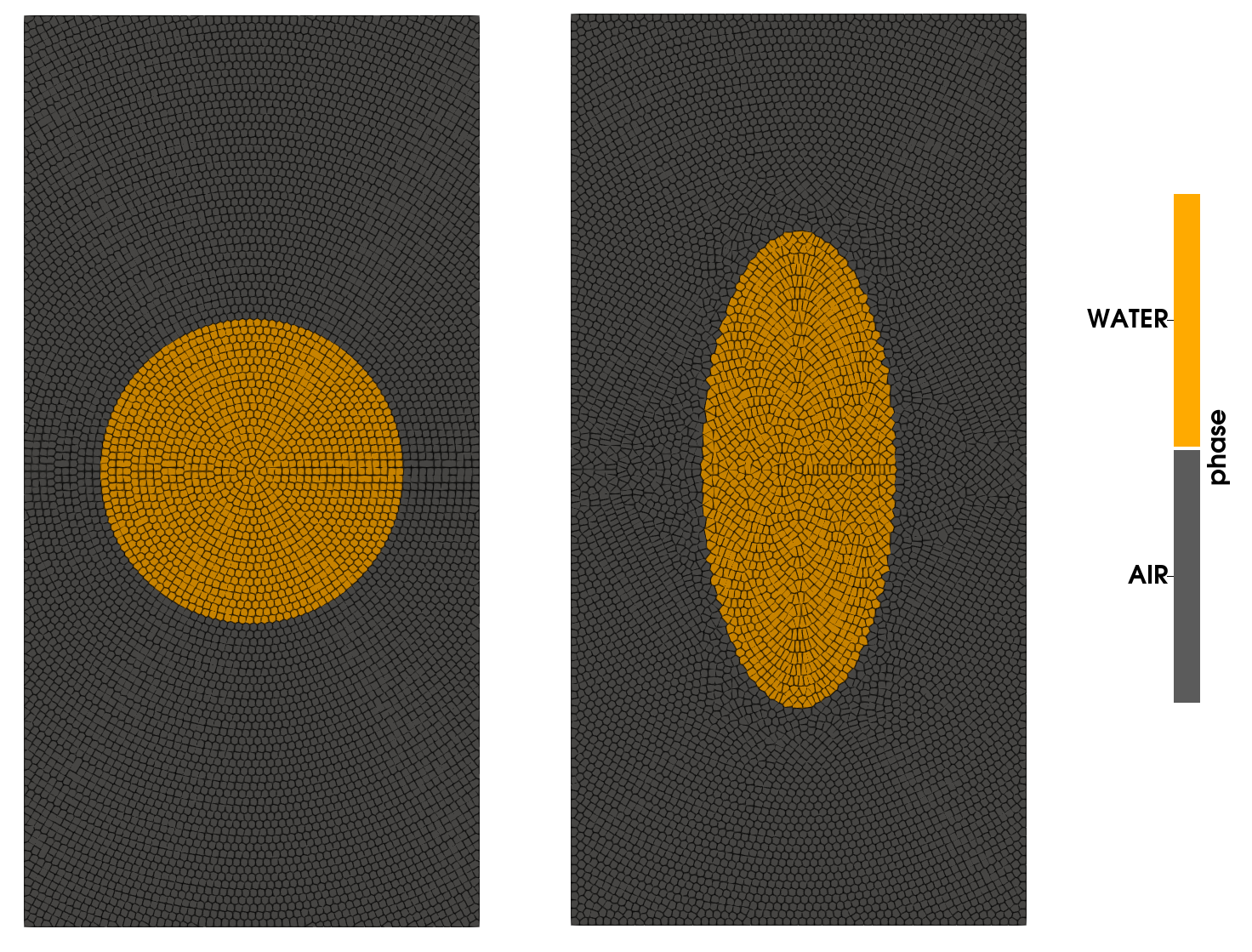
Circular patch is a free surface benchmark which admits a semi-analytical solution. Initially, there is a circle of radius 1 with some prescribed velocity. The resulting velocity deformation squeezes the patch. Now, we cannot do free surface with this code, but we can find a reasonable good solution by turning it into a multiphase problem where the surrounding air has much lower density.

module cpatch

include("../src/LagrangianVoronoi.jl")
using .LagrangianVoronoi

using DifferentialEquations
using StaticArrays
using Plots
using Parameters
using Base.Threads
using WriteVTK
using LinearAlgebra
using Polyester
using LaTeXStrings, CSV, DataFrames

const A0 = 0.5
const R = 1.0
const Rho = 1000.0
const rho = Rho/800
const dr = R/20

const v_char = A0*R
const dt = 0.1*dr/v_char
const t_end =  1.0
const nframes = 100
const tau = 0.1
const c0 = 100.0
const smoothing_length = 3dr

const export_path = "results/cpatch"
const xlims = (-1.5R, 1.5R)
const ylims = (-3.0R, 3.0R)

const WATER = 0
const AIR = 1

function ic!(p::VoronoiPolygon, e)
    p.c2 = Inf
    r = norm(p.x)
    p.phase = (r < R) ? WATER : AIR
    p.rho = (p.phase == WATER ? Rho : rho)
    p.mass = p.rho*area(p)
    if (p.phase == WATER)
        p.v = v_exact(p.x, e(0.0))
        p.P = P_exact(p.x, e(0.0))
    end
end

mutable struct Simulation <: SimulationWorkspace
    grid::GridMulti
    solver::PressureSolver{PolygonMulti}
    E::Float64  # total energy
    v_err::Float64 # L^2 error
    P_err::Float64
    e::Any # function that describes the exact evolution of the ellipse
    Simulation() = begin
        ode = ODEProblem(ellipse_ode, [R, R, A0], (0.0, t_end))
        e = solve(ode, Rodas4(), reltol = 1e-8, abstol = 1e-8)
        domain = Rectangle(xlims = xlims, ylims = ylims)
        grid = GridMulti(domain, dr)
        populate_circ!(grid, ic! = (p -> ic!(p, e)))
        solver = PressureSolver(grid, verbose=false)
        return new(grid, solver, 0.0, 0.0, 0.0, e)
    end
end

function ellipse_ode(e, _, _)
    return [
        -e[3]*e[1],
        +e[3]*e[2],
        (e[3]^2)*(e[1]^2 - e[2]^2)/(e[1]^2 + e[2]^2)
    ]
end

function v_exact(x::RealVector, e)::RealVector
    return RealVector(-e[3]*x[1], e[3]*x[2])
end

function P_exact(x::RealVector, e)::Float64
    return -Rho*(e[1]*e[2]*e[3])^2/(e[1]^2 + e[2]^2)*((x[1]/e[1])^2 + (x[2]/e[2])^2 - 1.0)
end

function step!(sim::Simulation, t::Float64)
    move!(sim.grid, dt)
    find_rho!(sim.grid)
    find_pressure!(sim.solver, dt)
    pressure_step!(sim.grid, dt)
    phase_preserving_remapping!(sim.grid, dt, smoothing_length)
end

function postproc!(sim::Simulation, t::Float64)
    sim.v_err = 0.0
    sim.P_err = 0.0
    sim.E = 0.0
    max_v_err = 0.0
    max_P_err = 0.0
    P_avg = 0.0
    A_tot = 0.0
    for p in sim.grid.polygons
        if (p.phase == AIR) continue end
        A = area(p)
        et = sim.e(t)
        sim.v_err += A*norm_squared(p.v - v_exact(p.x, et))
        max_v_err += A*norm_squared(v_exact(p.x, et))
        P_avg += A*(p.P - P_exact(p.x, et))
        A_tot += A
        max_P_err += A*P_exact(p.x, et)^2
        sim.E += p.mass*norm_squared(p.v)
    end
    P_avg /= A_tot
    for p in sim.grid.polygons
        if (p.phase == AIR) continue end
        A = area(p)
        et = sim.e(t)
        sim.P_err += A*(p.P - P_exact(p.x, et) - P_avg)^2
    end
    sim.P_err = sqrt(sim.P_err)/sqrt(max_P_err)
    sim.v_err = sqrt(sim.v_err)/sqrt(max_v_err)
    @show t
    @show sim.v_err
    @show sim.P_err
    @show sim.E
    println()
end


function main()
    sim = Simulation()
    run!(sim, dt, t_end, step!;
        path = export_path,
        postproc! = postproc!,
        vtp_vars = (:v, :P, :rho, :phase),      # local variables exported into vtp
        csv_vars = (:E, :v_err, :P_err),          # global variables exported into csv
        nframes = nframes,                # number of time frames
        save_points = true
    )
end

function linear_regression(x, y)
    N = length(x)
    logx = log10.(x)
    logy = log10.(y)
    A = [logx ones(N)]
    b = A\logy
    return b
end

function make_convergence_graph()
    data = CSV.read(joinpath(export_path, "convergence_data.csv"), DataFrame)
    x = log10.(data.N)
    y = [log10.(data.P) log10.(data.v)]
    eoc_p = linear_regression(data.N, data.P)[1]
    eoc_v = linear_regression(data.N, data.v)[1]
    xlabel = L"\log N"
    ylabel = L"\log \epsilon"
    p_label = L"p"*"   (EOC = $(-round(eoc_p, digits=2)))"
    v_label = L"v"*"   (EOC = $(-round(eoc_v, digits=2)))"
    plt = plot(x, y, xlabel=xlabel, ylabel=ylabel, label = [p_label v_label], marker = :hex, axis_ratio = 1.0)
    savefig(plt, joinpath(export_path, "convergence.pdf"))
end

end

This page was generated using Literate.jl.