Example 4: Double Shear Layer

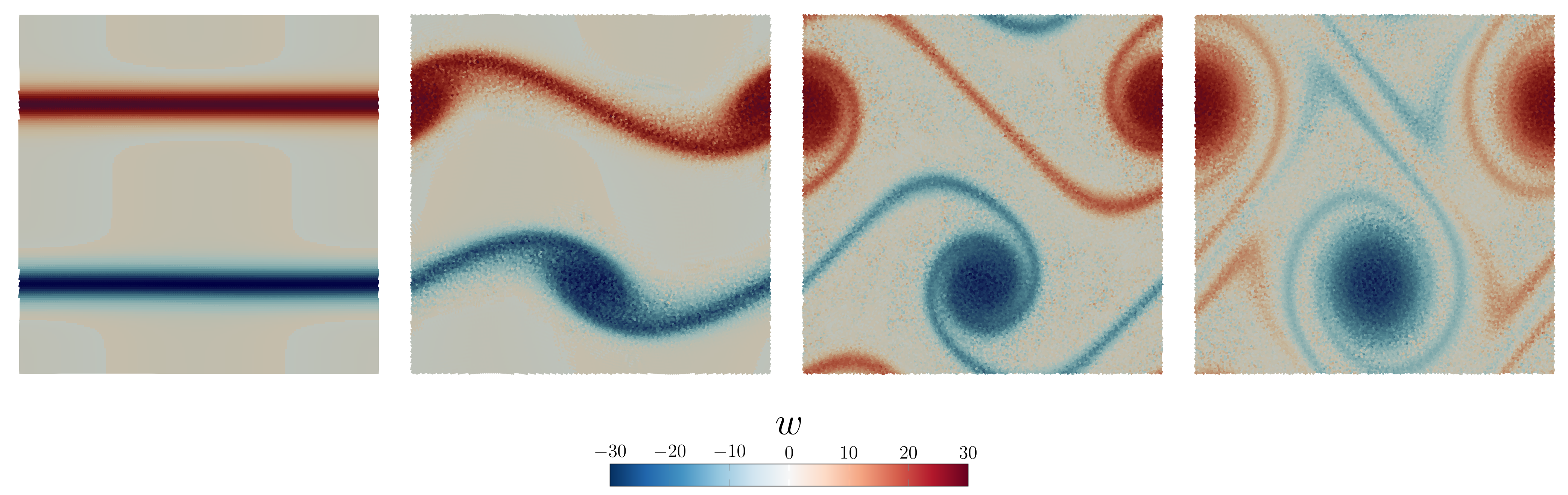
In this setup, borrowed from this paper, we consider a periodic domain and an initial velocity field

$u = \tanh\left(\xi \left(y - \frac{1}{4}\right) \right), \quad y < \frac{1}{2}$

$u = \tanh\left(\xi \left(\frac{3}{4} - y\right) \right), \quad y \geq \frac{1}{2}$

$v = \delta \sin(2 \pi x)$

with $\delta = 0.05$, $\xi = 30$, with constant initial density $\rho_0 = 1$, viscosity $\mu = 2E-4$ and pressure $P_0 = \frac{1}{\gamma}.$ These conditions generate an interesting flow pattern, which is essentially a Kelvin-Helmholtz instability. The problem relies on a periodic boundary condition which must be specified in the VoronoiGrid constructor.

module doubleshear
include("../src/LagrangianVoronoi.jl")
using .LagrangianVoronoi, LinearAlgebra, Polyester

const rho0 = 1.0
const xlims = (0.0, 1.0)
const ylims = (0.0, 1.0)
const mu = 2e-4
const dr = 1e-2
const gamma = 1.4
const P0 = 100.0/gamma

const delta = 0.05
const xi = 30.0
const v_char = 2.0
const dt = 0.1*dr/v_char

const t_end = 1.8

const export_path = "results/doubleshear"
const nframes = 100

function ic!(p::VoronoiPolygon)
    p.v = v_init(p.x)
    p.rho = rho0
    p.mass = p.rho*area(p)
    p.P = P0
    p.e = 0.5*norm_squared(p.v) + p.P/(p.rho*(gamma - 1.0))
    p.mu = mu
end

function v_init(x::RealVector)::RealVector
    u =  (x[2] <= 0.5) ? tanh(xi*(x[2] - 0.25)) : tanh(xi*(0.75 - x[2]))
    v = delta*sin(2pi*x[1])
    return RealVector(u,v)
end

In this example, we would like to compute vorticity. Unfortunately, the predefined Navier-Stokes polygon is not equipped with a vorticity field. However, we can create our custom type PolygonWithVorticity and perform all computations with it.

@kwdef mutable struct PolygonWithVorticity <: VoronoiPolygon
    @Euler_vars           # all standard variables
    D::RealMatrix = MAT0  # velocity deformation tensor
    mu::Float64 = 0.0     # dynamic viscosity
    vort::Float64 = 0.0   # vorticity
end

const GridWithVorticity = VoronoiGrid{PolygonWithVorticity}

mutable struct Simulation <: SimulationWorkspace
    grid::GridWithVorticity
    solver::PressureSolver{PolygonWithVorticity}
    E::Float64
    S::Float64
    E0::Float64
    S0::Float64
    first_step::Bool
    Simulation() = begin
        domain = Rectangle(xlims = xlims, ylims = ylims)
        grid = GridWithVorticity(domain, dr, xperiodic = true, yperiodic = true) # the domain is periodic both horizontally and vertically
        populate_lloyd!(grid, ic! = ic!)
        solver = PressureSolver(grid)
        return new(grid, solver, 0.0, 0.0, 0.0, 0.0, true)
    end
end

We need to define a custom function for vorticity evaluation. The vorticity can be evauluated using moving least squares. (Also known as "linear reconstruction" in some circles.) This is not the only way how vorticity can be approximated.

function get_vort!(grid::GridWithVorticity)
    @batch for p in grid.polygons
        gradu = movingls(LinearExpansion, grid, p, p -> p.v[1])
        gradv = movingls(LinearExpansion, grid, p, p -> p.v[2])
        p.vort = gradv[1] - gradu[2]
    end
end

The remainder of the script is as usual.

function step!(sim::Simulation, t::Float64)
    move!(sim.grid, dt)
    ideal_eos!(sim.grid, gamma)
    find_pressure!(sim.solver, dt)
    pressure_step!(sim.grid, dt)
    find_D!(sim.grid)
    viscous_step!(sim.grid, dt)
    find_dv!(sim.grid, dt)
    relaxation_step!(sim.grid, dt)
    return
end

function postproc!(sim::Simulation, t::Float64)
    get_vort!(sim.grid)
    @show t
    grid = sim.grid
    sim.E = 0.0
    sim.S = 0.0
    for p in grid.polygons
        sim.E += p.mass*p.e
        sim.S += p.mass*(log(abs(p.P/P0)) - gamma*log(abs(p.rho/rho0)))
    end
    if sim.first_step
        sim.E0 = sim.E
        sim.S0 = sim.S
        sim.first_step = false
    end
    sim.E -= sim.E0
    sim.S -= sim.S0
    @show sim.E
    @show sim.S
    println()
    return
end

function main()
    sim = Simulation()
    run!(sim, dt, t_end, step!;
        postproc! = postproc!,
        nframes = nframes,
        path = export_path,
        save_csv = false,
        save_points = true,
        save_grid = true,
        vtp_vars = (:P, :v, :rho, :vort)
    )
end

if abspath(PROGRAM_FILE) == @__FILE__
    main()
end

end

This page was generated using Literate.jl.