Example 8: Saltzman piston test

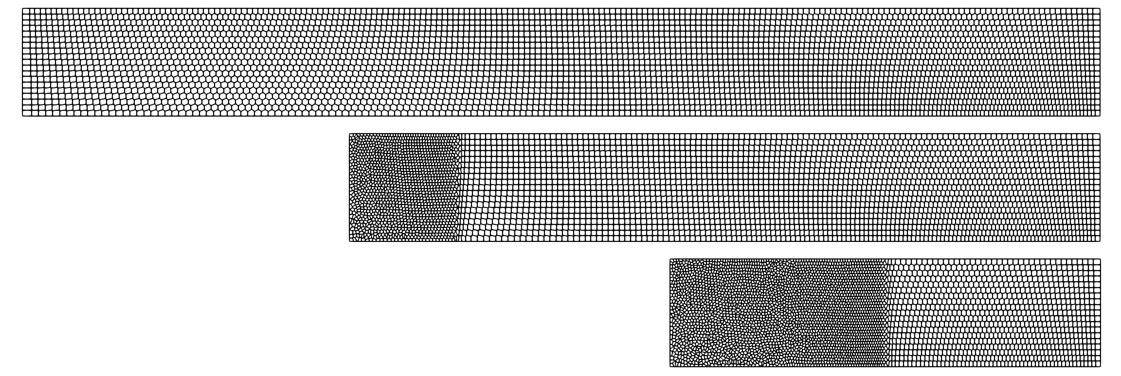
In this challenging test, the domain will vary with time. We study a piston of length 1 and width 0.1 filled with ideal gas which is initially at rest. Starting from $t=0$, the piston is compressed at a uniform rate at speed equal to 1. This produces a strong shockwave, whose characteristics can be computed analytically from Rankine-Hugeniot conditions. The simulation is terminated at $t = t_end$. Unknown things will happen if $t_end >= 1.0$, maybe it will even destroy the universe!

module piston
include("../src/LagrangianVoronoi.jl")
using .LagrangianVoronoi, WriteVTK, LinearAlgebra, Polyester
using LaTeXStrings, DataFrames, CSV, Plots, Measures, Match

const xlims = (0.0, 1.0)
const ylims = (0.0, 0.1)
const rho0 = 1.0
const P0 = 1e-4
const gamma = 5/3
const dr = 1/100

const CFL_early = 0.1
const t_early = 0.01
const CFL = 0.1

const t_end = 0.6
const nframes = 100

const export_path = "results/piston"

function ic!(p::VoronoiPolygon)
    p.rho = rho0
    p.mass = p.rho*area(p)
    p.P = P0
    p.e = 0.5*norm_squared(p.v) + p.P/(p.rho*(gamma - 1.0))
end

function cut_domain!(grid::VoronoiGrid, t::Float64)
    rect = Rectangle(xlims = (t, 1.0), ylims = ylims)
    grid.boundary_rect = rect
    grid.cropping_rect = rect
    remesh!(grid)
    @batch for p in grid.polygons

change density adiabatically

        if isleftbdarycell(p)
            rho_old = p.rho
            P_old = p.P
            p.rho = p.mass/area(p)
            p.P = P_old*(p.rho/rho_old)^gamma
            p.e = 0.5*norm_squared(p.v) + p.P/(p.rho*(gamma - 1.0))
        end
    end
end

function isleftbdarycell(p::VoronoiPolygon)::Bool
    for e in boundaries(p)
        if e.label == BDARY_LEFT
            return true
        end
    end
    return false
end

function dirichlet_bc!(grid::VoronoiGrid)
    @batch for p in grid.polygons
        if isleftbdarycell(p)
            p.v = VECX + p.v[2]*VECY
            p.e = 0.5*norm_squared(p.v) + p.P/(p.rho*(gamma - 1.0))
        end
    end
end


function move_points!(grid::VoronoiGrid,  t::Float64, dt::Float64)
    @batch for p in grid.polygons
        p.x += dt*p.v
    end
    remesh!(grid)
end


function populate_skewed!(grid::VoronoiGrid{T}; ic!::Function) where T <: VoronoiPolygon
    N = round(Int, 1.0/grid.dr)
    M = round(Int, 0.1/grid.dr)
    for x1 in range(-1.0, 2.0, 3N)
        for x2 in range(0.0, 0.1, M)
            x = RealVector(x1, x2) + 0.5*RealVector(grid.dr, grid.dr)
            x = RealVector(x[1] + (0.1 - x[2])*sin(pi*x[1]), x[2])
            if isinside(grid.boundary_rect, x)
                push!(grid.polygons, T(x=x))
            end
        end
    end
    remesh!(grid)
    @batch for p in grid.polygons
        ic!(p)
    end
	return
end

mutable struct Simulation <: SimulationWorkspace
    grid::GridNS
    solver::PressureSolver
    E::Float64
    S::Float64
    t::Float64
    Simulation() = begin
        domain = Rectangle(xlims = xlims, ylims = ylims)
        grid = GridNS(domain, dr)
        populate_skewed!(grid, ic! = ic!)
        solver = PressureSolver(grid)
        dirichlet_bc!(grid)
        return new(grid, solver, 0.0, 0.0, 0.0)
    end
end

function vbc(_::RealVector, bdary::Int)::RealVector
    if bdary == BDARY_LEFT
        return VECX
    end
    return VEC0
end


function step!(sim::Simulation)
    dt = (sim.t < t_early ? CFL_early : CFL)*dr
    ideal_eos!(sim.grid, gamma; Pmin = P0)
    find_pressure!(sim.solver, dt; boundary_velocity = vbc)
    pressure_step!(sim.grid, dt)
    find_D!(sim.grid)
    viscous_step!(sim.grid, dt)
    find_dv!(sim.grid, dt, 1.0)
    relaxation_step!(sim.grid, dt)
    dirichlet_bc!(sim.grid)
    move_points!(sim.grid, sim.t, dt)
    sim.t += dt
    cut_domain!(sim.grid, sim.t)
    return
end

Let us plot the total energy and entropy.

function postproc!(sim::Simulation)
    sim.E = 0.0
    sim.S = 0.0
    for p in sim.grid.polygons
        sim.E += p.mass*p.e
        sim.S += p.mass*log(abs(p.P/abs(p.rho)^gamma))
    end
    println("t = $(sim.t)")
    println("energy = $(sim.E)")
    println("entropy = $(sim.S)")
    println()
end

function main()
    if !ispath(export_path)
        mkpath(export_path)
        @info "created a new path: $(export_path)"
    end
    pvd_c = paraview_collection(joinpath(export_path, "cells.pvd"))
    pvd_p = paraview_collection(joinpath(export_path, "points.pvd"))
    nframe = 0
    sim = Simulation()
    milestones = collect(range(t_end, 0.0, nframes)) # save the data here
    vtp_vars = (:rho, :v, :e, :P, :phase, :mass)
    while sim.t < t_end
        step!(sim)
        if sim.t > milestones[end]
            @show sim.t
            postproc!(sim)
            println()
            filename= joinpath(export_path, "cframe$(nframe).vtp")
            pvd_c[sim.t] = export_grid(sim.grid, filename, vtp_vars...)
            filename= joinpath(export_path, "pframe$(nframe).vtp")
            pvd_p[sim.t] = export_points(sim.grid, filename, vtp_vars...)
            pop!(milestones)
            nframe += 1
        end
    end
    vtk_save(pvd_c)
    vtk_save(pvd_p)

    x = range(0.6, 1.0, 200)
    rho = [point_value(sim.grid, RealVector(_x, 0.05), p -> p.rho) for _x in x]
    P = [point_value(sim.grid, RealVector(_x, 0.05), p -> p.P) for _x in x]
    v = [point_value(sim.grid, RealVector(_x, 0.05), p -> p.v[1]) for _x in x]

    csv_data = DataFrame(x=x, rho=rho, P=P, v=v)
	CSV.write(string(export_path, "/linedata.csv"), csv_data)
    plotdata()
    print_l1_error(sim.grid)
    println()
    print_l2_error(sim.grid)
end

function plotdata()
    for var in (:rho, :P, :v)
        plotdata(var)
    end
end

function plotdata(var::Symbol)
    csv_data = CSV.read(string(export_path, "/linedata.csv"), DataFrame)
    x_shock = 0.8
    x_exact = [t_end, x_shock, nextfloat(x_shock), 1.0]
    y_sim, ylabel, y0, y1, color = @match var begin
        :rho => (csv_data.rho, L"\rho", 4.0, 1.0, :orange)
        :P => (csv_data.P, L"P", 2*(gamma-1.0), P0, :royalblue)
        :v => (csv_data.v, L"v", 1.0, 0.0, :teal)
    end
    y_exact = [(x <= x_shock ? y0 : y1) for x in x_exact]
    plt = plot(
        x_exact,
        y_exact,
        label = "EXACT",
        linewidth = 2,
        color = :black,
        xlabel = L"x",
        ylabel = ylabel,
        bottom_margin = 5mm,
        ylims = (0.0, max(y0,y1) + 0.5)
    )
    plot!(plt,
            csv_data.x,
            y_sim,
            label = "SIMULATION",
            markerstrokewidth = 1,
            markersize = 3,
            color = color,
            marker = :circ
    )
    savefig(plt, string(export_path, "/$(string(var)).pdf"))
    return
end

function print_l1_error(grid::VoronoiGrid)
    x_shock = 0.8
    for var in (:rho, :P, :v)
        err = 0.0
        y0, y1 = @match var begin
            :rho => (4.0, 1.0)
            :P => (2*(gamma-1.0), P0)
            :v => (1.0, 0.0)
        end
        for p in grid.polygons
            A = area(p)
            y = (p.x[1] <= x_shock ? y0 : y1)
            if (var != :v)
                err += A*abs(getproperty(p, var) - y)
            else
                err += A*abs(getproperty(p, var)[1] - y)
            end
        end
        println("$(var): l1 error = $(err)")
    end
end

function print_l2_error(grid::VoronoiGrid)
    x_shock = 0.8
    for var in (:rho, :P, :v)
        err = 0.0
        y0, y1 = @match var begin
            :rho => (4.0, 1.0)
            :P => (2*(gamma-1.0), P0)
            :v => (1.0, 0.0)
        end
        for p in grid.polygons
            A = area(p)
            y = (p.x[1] <= x_shock ? y0 : y1)
            if (var != :v)
                err += A*abs(getproperty(p, var) - y)^2
            else
                err += A*abs(getproperty(p, var)[1] - y)^2
            end
        end
        println("$(var): l2 error = $(sqrt(err))")
    end
end

function linear_regression(x, y)
    N = length(x)
    logx = log10.(x)
    logy = log10.(y)
    A = [logx ones(N)]
    b = A\logy
    return b
end

function make_convergence_graph()
    data = CSV.read(joinpath(export_path, "l2_convergence_data.csv"), DataFrame)
    x = log10.(data.N)
    y = [log10.(data.rho) log10.(data.P) log10.(data.v)]
    eoc_rho = linear_regression(data.N, data.rho)[1]
    eoc_p = linear_regression(data.N, data.P)[1]
    eoc_v = linear_regression(data.N, data.v)[1]
    xlabel = L"\log N"
    ylabel = L"\log \epsilon"
    rho_label = L"\rho"*"   (EOC = $(-round(eoc_rho, digits=2)))"
    p_label = L"p"*"   (EOC = $(-round(eoc_p, digits=2)))"
    v_label = L"v"*"   (EOC = $(-round(eoc_v, digits=2)))"
    plt = plot(x, y, xlabel=xlabel, ylabel=ylabel, label = [rho_label p_label v_label], marker = :hex, axis_ratio = 1.0)
    savefig(plt, joinpath(export_path, "l2_convergence.pdf"))
end

end

This page was generated using Literate.jl.